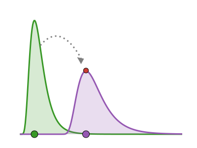
Convolving modified distributions

Introduction

ConvolvedDistributions.jl does two related jobs: it sums independent delays into a single total-delay distribution, and it convolves a numeric count series with a delay's discretised PMF to give expected downstream counts. Loading it alongside ModifiedDistributions activates a package extension that lets the modifiers ride both jobs: forward-series transforms (thin, cumulative, series_transform) act on the convolved counts, and modified distributions serve as convolution components.

What are we going to do in this exercise

2. Build a two-stage total delay and convolve an infection series with it.

3. Thin the convolved series with thin (ascertainment).

4. Accumulate it with cumulative (cumulative incidence).

5. Time-scale a convolved delay with affine.

6. See that a series op attached between two fused delays is ignored at the distribution level.

7. Convolve a ComposedDistributions.jl delay chain through the same stack, so a composed chain, a series convolution and a modifier work together end to end.

What might I need to know before starting

This tutorial builds on the Getting started overview, the A modifier pipeline tutorial and the Modifiers across composed chains tutorial, and uses Distributions.jl, ConvolvedDistributions.jl, ComposedDistributions.jl and ModifiedDistributions.jl, with CairoMakie and AlgebraOfGraphics for the figure.

Packages used

Loading ConvolvedDistributions and ComposedDistributions activates the two package extensions; CairoMakie and AlgebraOfGraphics are used for plotting only.

using ModifiedDistributions, ConvolvedDistributions, Distributions
using ComposedDistributions
using CairoMakie, AlgebraOfGraphics

CairoMakie.activate!(type = "png", px_per_unit = 2)
set_theme!(theme_latexfonts(); fontsize = 14)

A convolved total delay and an infection series

An observed delay is often the sum of stages: here infection-to-onset plus onset-to-report. convolve_series fuses the two into one total-delay distribution, and its mean is the sum of the stage means.

onset = Gamma(2.0, 1.0)
report = LogNormal(0.5, 0.4)
total = convolved(onset, report)
(total_mean = mean(total), stage_sum = mean(onset) + mean(report))

(total_mean = 3.7860384307500734, stage_sum = 3.7860384307500734)

A continuous total delay carries no mass on the integer day grid until it is discretised, and ConvolvedDistributions 0.2 leaves that explicit modelling choice to the caller: discretise_pmf turns the total into a daily PMF, which convolve_series then convolves with the series. Feeding it an expected-infections curve gives the expected reported counts each day.

infections = [0.0, 10.0, 40.0, 90.0, 120.0, 100.0, 60.0, 30.0, 12.0, 4.0]
reported = convolve_series(
    discretise_pmf(total, length(infections) - 1), infections)
reported

10-element Vector{Float64}:
  0.0
  0.018168681675718616
  1.0072468423757484
  6.516548917771465
 21.75868804496929
 47.425196658986316
 73.13508265857033
 84.74189473288018
 78.37740987664519
 60.93163463615561

Thinning the convolved counts (ascertainment)

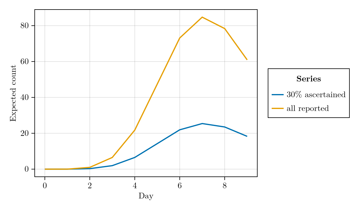
Only a fraction of events is usually observed. thin attaches that ascertainment fraction to the delay, and the extension applies it to the convolved counts: every day below is 0.3 times the unthinned baseline.

ascertained = convolve_series(thin(total, 0.3), infections)
(day4_thinned = ascertained[4], day4_check = 0.3 * reported[4])

(day4_thinned = 1.9549646753314396, day4_check = 1.9549646753314396)

Plotting the baseline against the thinned series shows the op acting on the whole curve at once.

days = collect(0:(length(infections) - 1))
series_curves = (
    day = vcat(days, days),
    count = vcat(reported, ascertained),
    series = vcat(fill("all reported", length(days)),
        fill("30% ascertained", length(days)))
)
draw(
    data(series_curves) *
    mapping(:day => "Day", :count => "Expected count",
        color = :series => "Series") *
    visual(Lines, linewidth = 2);
    figure = (size = (600, 350),)
)

Cumulative incidence

cumulative accumulates the convolved counts into a running total, so the final day below equals the sum of the whole daily series.

cumulative_counts = convolve_series(cumulative(total), infections)
(final_cumulative = cumulative_counts[end], daily_sum = sum(reported))

(final_cumulative = 373.91187105002984, daily_sum = 373.91187105002984)

The wrappers nest, applying innermost first: thinning then accumulating gives cumulative ascertained incidence.

cum_ascertained = convolve_series(
    thin(cumulative(total), 0.3), infections)
(final = cum_ascertained[end], check = 0.3 * sum(reported))

(final = 112.17356131500895, check = 112.17356131500895)

Time-scaling a convolved delay

affine wraps the total delay just as it wraps any univariate distribution, so a change of time unit (or a stretch of the delay) is a scale on the fused total. Doubling the delay doubles its mean, and the stretched delay pushes the convolved counts later and flatter.

stretched = affine(total; scale = 2.0)
(total_mean = mean(total), stretched_mean = mean(stretched))

(total_mean = 3.7860384307500734, stretched_mean = 7.572076861500147)

reported_stretched = convolve_series(stretched, infections)
(peak_day_base = days[argmax(reported)],
    peak_day_stretched = days[argmax(reported_stretched)])

(peak_day_base = 7, peak_day_stretched = 9)

A series op between two fused delays is ignored at the distribution level

A forward op belongs to the wrapper it is attached to, and it only fires when THAT wrapper is handed a series. If a thinned stage is fused into a distribution-level convolution, the total delay's density is untouched: thin is transparent to every distribution method, so the fused CDF with and without the op agree exactly.

fused_plain = convolved(onset, report)
fused_thinned_stage = convolved(thin(onset, 0.3), report)
(cdf_plain = cdf(fused_plain, 4.0),
    cdf_with_op_inside = cdf(fused_thinned_stage, 4.0))

(cdf_plain = 0.6238028661157885, cdf_with_op_inside = 0.6238028661157885)

The printed CDFs are identical: the op sits inert between the two fused delays. To thin the OUTPUT of the fused delay, attach the op to the fused total itself (as in the ascertainment section above), where the series handshake can see it.

The full stack: a composed chain, convolved, then modified

The two extensions meet when a ComposedDistributions.jl delay chain is convolved through a series and a modifier reshapes the result. A Sequential links delay stages; observed_distribution collapses it to the single total delay a downstream observation sees, exactly the fused total used above (see the composed chains tutorial).

chain = sequential(:infect_onset => onset, :onset_report => report)
chain_total = observed_distribution(chain)
(chain_mean = mean(chain_total), fused_mean = mean(total))

(chain_mean = 3.7860384307500734, fused_mean = 3.7860384307500734)

A modifier on the chain wraps that collapsed total, and convolve_series then discretises it and applies the modifier's series op — the same handshake as for the fused total, so the two paths agree. Thinning the chain gives 0.3 times the baseline reported counts.

chain_ascertained = convolve_series(thin(chain, 0.3), infections)
(day4_chain = chain_ascertained[4], day4_check = 0.3 * reported[4])

(day4_chain = 1.9549646753314396, day4_check = 1.9549646753314396)

The bare collapsed total is a continuous distribution, so a direct convolve_series(chain_total, infections) would (rightly) refuse to discretise silently; the modifier convenience discretises for you, and an explicit discretise_pmf reproduces the same baseline.

chain_baseline = convolve_series(
    discretise_pmf(chain_total, length(infections) - 1), infections)
(via_modifier = convolve_series(thin(chain, 1.0), infections)[end],
    via_discretise = chain_baseline[end])

(via_modifier = 60.93163463615561, via_discretise = 60.93163463615561)

affine and cumulative ride the composed chain the same way, so a change of time unit and a running total compose with the chain too.

chain_cumulative = convolve_series(cumulative(chain), infections)
(final_cumulative = chain_cumulative[end], daily_sum = sum(chain_baseline))

(final_cumulative = 373.91187105002984, daily_sum = 373.91187105002984)

A Parallel has several independent endpoints and no single total delay, so convolve_series is applied to each branch's endpoint rather than the whole node; convolve event(modified_parallel, name) per branch.

Summary

• convolve_series(delay, series) turns an infection series into expected downstream counts, and the extension lets thin, cumulative and series_transform act on those counts.

• Wrappers nest and apply innermost first.

• affine time-scales a fused total delay like any other distribution, and modified distributions can sit inside a convolution.

• A series op fused between two delays is ignored at the distribution level; attach it to the object that receives the series.

• A composed Sequential chain collapses to its total delay, so the whole stack — chain, series convolution and modifier — works end to end; a Parallel is convolved branch by branch.