Modifiers across composed chains

Introduction

ComposedDistributions.jl builds chains of distributions: a Sequential links a series of steps, and the whole chain observes one scalar quantity, the convolved total of its steps. When ComposedDistributions is loaded alongside ModifiedDistributions a package extension lets the modifier verbs apply to a chain directly. A modifier on a chain modifies that observed scalar: the chain collapses to its convolved total first, then the modifier wraps the resulting univariate distribution.

What are we going to do in this exercise

1. Build a Sequential chain and collapse it with observed_distribution.

2. Apply weight, affine and thin to the chain and check the modifier lands on the chain's observed scalar.

3. See how this package and ComposedDistributions.jl split the work between them.

What might I need to know before starting

This tutorial builds on the Getting started overview and the modifier pipeline tutorial. It additionally needs ComposedDistributions.jl, which is pinned in the docs environment.

Packages used

Loading ComposedDistributions activates the extension; no extra import is needed to reach the modifier methods for a chain. CairoMakie and AlgebraOfGraphics are used for plotting only.

using ModifiedDistributions, Distributions
using ComposedDistributions
using CairoMakie, AlgebraOfGraphics

CairoMakie.activate!(type = "png", px_per_unit = 2)
set_theme!(theme_latexfonts(); fontsize = 14)

A sequential chain and its observed scalar

A Sequential chain of two delays represents, say, onset to admission and admission to death. Its realisation is a vector of step values, so a chain is a multivariate distribution.

chain = sequential(:onset_admit => Gamma(2.0, 1.0),
    :admit_death => LogNormal(0.5, 0.4))
event_names(chain)

(:onset, :admit, :death)

A downstream observation sees one quantity: the total elapsed time from origin to the terminal event, the convolution of the steps. observed_distribution lowers the chain to that univariate scalar (we show its type — printing the full object dumps its quadrature internals).

observed = observed_distribution(chain)
typeof(observed)

ConvolvedDistributions.Convolved{Tuple{Distributions.Gamma{Float64}, Distributions.LogNormal{Float64}}, ConvolvedDistributions.AnalyticalSolver{ConvolvedDistributions.GaussLegendre{ConvolvedDistributions._GL{Vector{Float64}, Vector{Float64}}}}}

A modifier lands on the observed scalar

weight on the chain weights the observed total. The extension collapses the chain to observed and weights that, so the two log-densities printed below match: weighting the chain is weighting the observed scalar.

wd = weight(chain, 3.0)
(weighted_chain = logpdf(wd, 5.0), manual = 3.0 * logpdf(observed, 5.0))

(weighted_chain = -5.969634604903704, manual = -5.969634604903704)

Unwrapping the weighted chain with get_dist recovers a univariate distribution, the observed scalar, rather than the multivariate chain.

unwrapped = get_dist(wd)
typeof(unwrapped)

ConvolvedDistributions.Convolved{Tuple{Distributions.Gamma{Float64}, Distributions.LogNormal{Float64}}, ConvolvedDistributions.AnalyticalSolver{ConvolvedDistributions.GaussLegendre{ConvolvedDistributions._GL{Vector{Float64}, Vector{Float64}}}}}

It behaves like the collapsed total: the two log-densities printed below are identical.

(unwrapped = logpdf(unwrapped, 5.0), observed = logpdf(observed, 5.0))

(unwrapped = -1.989878201634568, observed = -1.989878201634568)

affine reparameterises the observed total the same way, matching the affine transform of the collapsed distribution.

ad = affine(chain; scale = 2.0, shift = 1.0)
(affine_chain = logpdf(ad, 10.0),
    manual = logpdf(affine(observed; scale = 2.0, shift = 1.0), 10.0))

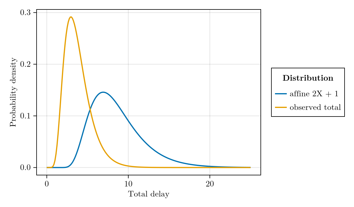
(affine_chain = -2.403753835465413, manual = -2.403753835465413)

Plotting the observed total's density next to its affine transform shows the modifier acting on the chain's one observed quantity: the transformed density is stretched, shifted and lowered relative to the total.

ts = collect(range(0.0, 25.0; length = 200))
total_curves = (
    t = vcat(ts, ts),
    density = vcat(pdf.(observed, ts), pdf.(ad, ts)),
    dist = vcat(fill("observed total", length(ts)),
        fill("affine 2X + 1", length(ts)))
)
draw(
    data(total_curves) *
    mapping(:t => "Total delay", :density => "Probability density",
        color = :dist => "Distribution") *
    visual(Lines, linewidth = 2);
    figure = (size = (600, 350),)
)

thin attaches a forward-series op to the chain's observed total and stays transparent to logpdf, exactly as it does for a plain distribution: the two log-densities printed below are identical.

td = thin(chain, 0.3)
(thinned = logpdf(td, 5.0), observed = logpdf(observed, 5.0))

(thinned = -1.989878201634568, observed = -1.989878201634568)

The observation-time weight forms carry over too, since they are defined on the collapsed scalar; the printed pair matches again.

wd_obs = weight(chain)
(observation_time = logpdf(wd_obs, (value = 5.0, weight = 3.0)),
    manual = 3.0 * logpdf(observed, 5.0))

(observation_time = -5.969634604903704, manual = -5.969634604903704)

How the two packages fit together

The extension in this package handles the forward direction: a modifier applied to a whole chain modifies the scalar the chain observes. The reverse direction — rewrapping modifier leaves sitting inside a composed tree (free_leaf / rewrap_leaf and shared tags) — lives in ComposedDistributions.jl, so a chain built from already modified steps composes correctly there. The split follows package ownership: this package owns the modifier verbs, ComposedDistributions owns the chain types, and each extension lives with the package that depends on both, so neither commits type piracy. A Parallel has several independent endpoints and so no single observed scalar, so the modifier verbs are not defined for it.

Summary

• observed_distribution collapses a Sequential chain to the univariate total it observes.

• weight, affine and thin on a chain modify that observed scalar, matching the modifier applied to the collapsed distribution.

• This package applies modifiers to a chain; ComposedDistributions.jl handles modifier leaves inside a chain, so modifiers compose with chains from either side.