Public Documentation
Documentation for ModifiedDistributions's public interface.
ModifiedDistributions.ModifiedDistributions Module
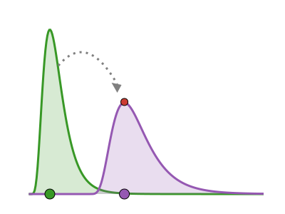
ModifiedDistributionsUnary modifiers that wrap exactly one UnivariateDistribution from Distributions.jl: an affine transform (affine), a likelihood weight (weight), and forward-series transforms (thin / cumulative). Also owns the generic get_dist unwrap protocol.
When ComposedDistributions.jl is loaded, a package extension additionally lets the modifier verbs apply across a composed Sequential chain by modifying the univariate scalar the chain observes (its convolved total).
Examples
using ModifiedDistributions, Distributions

d = affine(LogNormal(1.5, 0.5); scale = 2.0, shift = 1.0)
wd = weight(d, 10.0)
get_dist(wd) === dContents
Index
ModifiedDistributions.ModifiedDistributionsModifiedDistributions.IdentityLinkModifiedDistributions.LogLinkModifiedDistributions.LogitLinkModifiedDistributions.AbstractModifiedDistributionModifiedDistributions.AffineModifiedDistributions.CumulativeOpModifiedDistributions.HazardLinkModifiedDistributions.ModifiedModifiedDistributions.ThinOpModifiedDistributions.TransformedModifiedDistributions.WeightedModifiedDistributions.affineModifiedDistributions.apply_hazard_effectsModifiedDistributions.cumulativeModifiedDistributions.delay_hazardModifiedDistributions.effective_intensityModifiedDistributions.get_distModifiedDistributions.get_dist_recursiveModifiedDistributions.get_effectModifiedDistributions.get_factorModifiedDistributions.get_linkModifiedDistributions.get_opModifiedDistributions.get_scaleModifiedDistributions.get_shiftModifiedDistributions.get_weightModifiedDistributions.hazard_linkModifiedDistributions.hazard_to_pmfModifiedDistributions.intensityModifiedDistributions.is_defectiveModifiedDistributions.modifyModifiedDistributions.series_transformModifiedDistributions.thinModifiedDistributions.total_massModifiedDistributions.weight
Public API
ModifiedDistributions.AbstractModifiedDistribution Type
abstract type AbstractModifiedDistribution{F<:Distributions.VariateForm, S<:Distributions.ValueSupport} <: Distributions.Distribution{F<:Distributions.VariateForm, S<:Distributions.ValueSupport}Supertype of the single-base modifier leaves that wrap one inner distribution and modify it: Affine, Weighted, Transformed, Modified. CensoredDistributions' TimeChange and Shared leaves stay upstream until the migration (CensoredDistributions#343) lands. Parametric on variate form for symmetry with the upstream hierarchy.
Required methods a concrete subtype implements (the leaf interface):
an inner base reachable as
.dist(the defaultshowaccessor; overrideModifiedDistributions._modified_innerif stored elsewhere) and viaget_dist;the univariate interface (
pdf/logpdf/cdf/quantile/minimum/maximum/insupport/params), forwarded or specialised;optionally
Base.show; the default below printsName(inner).
The free_leaf / rewrap_leaf round-trip verbs are ComposedDistributions.jl's generics, so they are not part of this package's contract. Their methods for modifier leaves live in this package's own ModifiedDistributionsComposedDistributionsExt, which loads automatically when ComposedDistributions.jl is present.
Verify a subtype with ModifiedDistributions.TestUtils.test_modified_interface.
Fields
sourceModifiedDistributions.Affine Type
struct Affine{D<:(Distributions.UnivariateDistribution), T<:Real, S<:Distributions.ValueSupport} <: ModifiedDistributions.AbstractModifiedDistribution{Distributions.Univariate, S<:Distributions.ValueSupport}The distribution of a deterministic affine transform Y = scale * X + shift of an inner distribution X, with scale > 0 and any real shift.
For a continuous inner distribution, computed by the change-of-variables for a strictly increasing affine map: with x = (y - shift) / scale,
For a discrete inner distribution, the probability mass moves to the rescaled lattice without the Jacobian term: P(Y = y) = P(X = (y - shift) / scale).
Affine is a UnivariateDistribution with the value support of the inner distribution, so it works anywhere a distribution is expected.
See also
affine: constructor function
Fields
dist::Distributions.UnivariateDistribution: The inner distribution being transformed.scale::Real: The positive multiplicative scale.shift::Real: The additive shift.
ModifiedDistributions.CumulativeOp Type
struct CumulativeOpThe forward op carried by cumulative: accumulate a downstream count series with a running sum.
See also
cumulative: the constructor verb.
Fields
sourceModifiedDistributions.HazardLink Type
struct HazardLink{G, GI}A link for the hazard modification carried by a Modified distribution.
The modification acts on the hazard through the link g,
so log gives proportional hazards and identity gives additive hazards. A HazardLink pairs the link g with its inverse invlink (g⁻¹); the three named links (LogLink, IdentityLink, LogitLink) are built-in, and any invertible callable can be wrapped with hazard_link. The log and identity links have analytic forms; a general link takes the numeric cumulative-hazard path, enabled by loading a quadrature backend (using QuadGK).
See also
Fields
g::Any: The linkgmapping a hazard onto the modification scale.invlink::Any: The inverse linkg⁻¹mapping back to a hazard.
ModifiedDistributions.IdentityLink Constant
IdentityLinkThe identity link (additive hazards): g = g⁻¹ = identity.
IdentityLink adds to the cumulative hazard from the support minimum m, m is required either way (see modify).
Examples
using ModifiedDistributions, Distributions

# Additive-hazards modification of an Exponential delay.
modify(Exponential(1.0), 0.5; link = ModifiedDistributions.IdentityLink)
See also
modify: the verb that consumes a link.HazardLink: the underlying link type.
ModifiedDistributions.LogLink Constant
LogLinkThe log link (proportional hazards): g = log, g⁻¹ = exp.
LogLink scales the survival function, modify.
Examples
using ModifiedDistributions, Distributions

# Proportional-hazards modification of an Exponential delay.
modify(Exponential(1.0), 0.5; link = ModifiedDistributions.LogLink)
See also
modify: the verb that consumes a link.HazardLink: the underlying link type.
ModifiedDistributions.LogitLink Constant
LogitLinkThe logit link (discrete-time reporting hazard): g = logit, g⁻¹ = logistic.
LogitLink pairs the logit with its logistic inverse, the link for a discrete-time reporting hazard on a discrete base with a per-bin effect vector, where each bin's hazard is a probability in (0, 1). On a continuous base the hazard is a rate that can exceed one, where the logit is not meaningful; the rate links LogLink and IdentityLink (or a custom hazard_link) are the continuous-base choices.
Examples
using ModifiedDistributions, Distributions

# A discrete-time reporting-hazard modification through LogitLink: a per-bin
# effect vector reshapes a discrete delay's hazard.
grid = collect(0:4)
base = DiscreteNonParametric(grid, fill(0.2, 5))
modify(base, fill(0.3, 5); link = ModifiedDistributions.LogitLink)
See also
modify: the verb that consumes a link.HazardLink: the underlying link type.
ModifiedDistributions.Modified Type
struct Modified{D<:(Distributions.UnivariateDistribution), E, L<:ModifiedDistributions.HazardLink, S<:Distributions.ValueSupport} <: ModifiedDistributions.AbstractModifiedDistribution{Distributions.Univariate, S<:Distributions.ValueSupport}A distribution whose hazard is modified through a link.
Modified carries a base distribution dist, a hazard effect and a HazardLink link, and lazily instantiates the modified hazard
in logpdf/cdf/ccdf/rand, where g is the link and h(t) = f(t)/S(t) the base hazard. The modification is never materialised eagerly, so a Modified composes with everything that consumes a UnivariateDistribution.
The effect is a scalar, a callable effect(t), or a per-bin AbstractVector, and the evaluation path is chosen by dispatch on the base and the link:
continuous base,
LogLinkwith a scalar effect: analytic proportional hazards,continuous base,
IdentityLinkwith a scalar effect and a finite lower support boundm: analytic additive hazards. A non-negative effect usesdiscrete base, per-bin vector effect: exact per-bin PMF reconstruction through the discrete-time reporting hazard, for any link;
continuous base, callable
effect(t)(any link) or a scalar effect under a general link: the modified cumulative hazardModifiedconstructs freely, but evaluating it needs a quadrature backend loaded (using QuadGK, supplied byModifiedDistributionsQuadGKExt); without one it throws anArgumentErrorpointing at the backend.
Every link works on a discrete base through the per-bin reconstruction.
Fields
dist: the base distribution whose hazard is modified.effect: the hazard modification (a scalar, a callableeffect(t), or a per-bin vector for a discrete base).link: the hazard linkgand its inverse.
See also
modify: the constructor verb.
Fields
dist::Distributions.UnivariateDistribution: The base distribution whose hazard is modified.effect::Any: The hazard modification effect (a scalar, a callableeffect(t), or a per-bin vector for a discrete base).link::ModifiedDistributions.HazardLink: The hazard linkgand its inverse.
ModifiedDistributions.ThinOp Type
struct ThinOp{T<:Real}The forward op carried by thin: multiply a downstream count series by a fixed factor (thinning / rescaling of expected counts). factor is the public field, so downstream packages can dispatch on Transformed{D, <:ThinOp} and read or rebuild the factor.
See also
thin: the constructor verb.
Fields
factor::Real: The fixed multiplicative factor applied to the series.
ModifiedDistributions.Transformed Type
struct Transformed{D<:(Distributions.UnivariateDistribution), Op, S<:Distributions.ValueSupport} <: ModifiedDistributions.AbstractModifiedDistribution{Distributions.Univariate, S<:Distributions.ValueSupport}A distribution carrying a forward-transform op, intended for a count series a downstream convolution layer produces. Transparent to logpdf and to every other distribution method (they delegate to the inner distribution). Construct with the generic series_transform or the specialised thin / cumulative.
See also
series_transform,thin,cumulative: constructors
Fields
dist::Distributions.UnivariateDistribution: The inner distribution.op::Any: The forward op applied to a convolved series.
ModifiedDistributions.Weighted Type
struct Weighted{D<:(Distributions.UnivariateDistribution), T<:Union{Missing, Real}, S<:Distributions.ValueSupport} <: ModifiedDistributions.AbstractModifiedDistribution{Distributions.Univariate, S<:Distributions.ValueSupport}A distribution wrapper that applies a weight to the log-probability of an underlying distribution. This is primarily used where observations have associated counts or weights.
Only the logpdf method is affected by the weight - all other methods (pdf, cdf, sampling, etc.) delegate directly to the underlying distribution.
Weight Types Supported
The Weighted struct supports three different weight scenarios: 2. Real weights: Constructor weight is a specific value (e.g., 2.5)
Missing weights: Constructor weight is
missing, allowing weights to be provided at observation time via joint observations(value = x, weight = w)Zero weights: Handled specially to return
-Infand avoid NaN from0 * -Inf
Examples
using ModifiedDistributions, Distributions

# Single weighted observation
d = LogNormal(1.5, 0.5)
wd = weight(d, 10.0)  # Observation with weight/count of 10

# Weighted log-probability calculation
observed_value = 2.0
weighted_logpdf = logpdf(wd, observed_value)

# Compare with manual calculation
manual_logpdf = 10.0 * logpdf(d, observed_value)
# weighted_logpdf ≈ manual_logpdf
Fields
dist::Distributions.UnivariateDistribution: The underlying distribution being weighted.weight::Union{Missing, Real}: The weight to apply to log-probabilities.
ModifiedDistributions.affine Function
affine(
    dist::Distributions.UnivariateDistribution;
    scale,
    shift
) -> ModifiedDistributions.Affine{D, Float64} where D<:(Distributions.UnivariateDistribution)
Create an affine-transformed distribution Y = scale * X + shift.
Arguments
dist: the inner distributionX.
Keyword Arguments
scale: positive multiplicative factor (default1).shift: additive offset (default0).
Examples
using ModifiedDistributions, Distributions

d = affine(LogNormal(1.5, 0.5); scale = 2.0, shift = 1.0)
logpdf(d, 5.0)
See also
Affine: the wrapped type
ModifiedDistributions.apply_hazard_effects Function
apply_hazard_effects(
    pmf::AbstractVector,
    effects::AbstractVector
) -> Any
Modify a delay PMF through its discrete-time hazard with additive logit effects.
apply_hazard_effects(pmf, effects) reshapes a baseline delay pmf by adding effects to its hazard on the logit scale and reconstructing the PMF,
the epinowcast logit-hazard model: a positive effect speeds reporting at that delay and the returned PMF is the modified per-reference-date delay distribution. The maximum-delay hazard stays one, so
The map is logit -> add -> logistic -> reconstruct, all AD-safe arithmetic, so Dual/tracked effects differentiate through.
Arguments
pmf: the baseline delay PMF over the grid0:D.effects: the additive logit-hazard effects, one per delay, same length as pmf. Use zeros for no modification.
Examples
using ModifiedDistributions

pmf = [0.2, 0.3, 0.3, 0.2]
# A positive early-delay effect speeds reporting at short delays.
effects = [0.8, 0.4, 0.0, 0.0]
ModifiedDistributions.apply_hazard_effects(pmf, effects)
See also
delay_hazard,hazard_to_pmf: the hazard <-> PMF maps.
ModifiedDistributions.cumulative Function
cumulative(
    dist::Distributions.UnivariateDistribution
) -> ModifiedDistributions.Transformed{D, ModifiedDistributions.CumulativeOp} where D<:(Distributions.UnivariateDistribution)
Accumulate a distribution's forward count series.
cumulative(d) is series_transform with a running-sum op intended for a downstream count series, giving cumulative counts (cumulative incidence, cumulative deaths). Transparent to logpdf. Under the ConvolvedDistributions extension the carried op applies to the convolved count series.
Arguments
d: the inner distribution.
Examples
using ModifiedDistributions, Distributions

d = cumulative(Gamma(2.0, 1.0))
logpdf(d, 2.0) == logpdf(Gamma(2.0, 1.0), 2.0)
See also
series_transform: the generic forward transformthin: a fixed forward factor
ModifiedDistributions.delay_hazard Function
delay_hazard(pmf::AbstractVector) -> AnyDiscrete-time reporting hazard of a delay PMF.
delay_hazard(pmf) converts a delay probability-mass vector pmf (the probability of report at each delay
the conditional probability of report at delay
The reduction is a cumulative sum and a divide, seeded from the input element type, so Dual/tracked numbers propagate and the hazard differentiates under AD.
Arguments
pmf: the delay PMF over the grid0:D.
Examples
using ModifiedDistributions

pmf = [0.2, 0.3, 0.3, 0.2]
ModifiedDistributions.delay_hazard(pmf)
See also
hazard_to_pmf: the inverse map (hazard -> PMF).apply_hazard_effects: add logit-scale per-bin effects.
ModifiedDistributions.effective_intensity Function
effective_intensity(tree, path::Tuple) -> AnyReturn the effective intensity of a declared factor within a composed tree.
The node at path's declared intensity, scaled by the probability its active period is reached and by the fraction of its kernel mass surviving the competing components above it in the tree. Equivalent to hand-integrating the component-resolved sub-density, but read straight off the tree. Needs ComposedDistributions.jl loaded to descend a non-empty path; an empty path reads tree itself, needing no tree machinery.
A Resolve/Compete ancestor discounts the reach by its branch probability. A Sequential/Parallel/Choose ancestor passes straight through with no discount. Every Sequential/Parallel child always executes, and a Choose alternative is picked by the data rather than a modelled probability. Do not sum effective_intensity across a Choose node's alternatives to get a combined intensity: only one alternative applies per record, so a caller summing over them double-counts.
Arguments
tree: the composed tree (or a bare node) to read.path: a tuple of edge names, the same formupdate/prune/spliceaccept, fromtreedown to the node whose factor to read.
Examples
using ModifiedDistributions, Distributions

node = thin(Gamma(2.0, 1.0), 0.3)
effective_intensity(node, ())
See also
intensity: the plain declared-factor reader (no tree context).
ModifiedDistributions.get_dist Function
get_dist(d) -> Distributions.UnivariateDistributionExtract the underlying distribution from a wrapped distribution type.
This protocol provides a consistent interface for extracting the core distribution from the modifier wrappers in this package (and any downstream wrapper that adds a method). For unwrapped distributions, it returns the distribution unchanged.
Arguments
d: A distribution or wrapped distribution.
Returns
The underlying distribution. For base distributions, returns d unchanged.
Examples
using ModifiedDistributions, Distributions

# Base distribution - returns unchanged
d1 = Normal(0, 1)
get_dist(d1)

# Affine-transformed distribution
d2 = affine(LogNormal(1.5, 0.5); scale = 2.0)
get_dist(d2)get_dist(
d::ModifiedDistributions.Affine
) -> Distributions.UnivariateDistributionExtract the underlying distribution from an affine-transformed distribution.
Returns the inner distribution before the affine transform was applied.
sourceget_dist(
d::ModifiedDistributions.Weighted
) -> Distributions.UnivariateDistributionExtract the underlying distribution from a weighted distribution.
Returns the base distribution before weighting was applied.
sourceget_dist(
d::ModifiedDistributions.Transformed
) -> Distributions.UnivariateDistributionExtract the underlying distribution from a forward-transformed distribution.
Returns the inner distribution before the forward-transform op was attached.
sourceget_dist(
d::ModifiedDistributions.Modified
) -> Distributions.UnivariateDistributionExtract the underlying distribution from a hazard-modified distribution.
Returns the base distribution before the hazard modification was applied.
sourceget_dist(
d::Distributions.Product
) -> AbstractVector{T} where {S<:Distributions.ValueSupport, T<:Distributions.UnivariateDistribution{S}}Extract the component distributions from a product distribution.
Returns a vector containing the underlying distribution of each component, so get_dist_recursive can unwrap vectorised forms such as weight(dist, weights).
Note
Unlike the other get_dist methods this returns a vector of distributions rather than a single distribution.
ModifiedDistributions.get_dist_recursive Function
get_dist_recursive(d) -> AnyRecursively extract the underlying distribution from nested wrapper types.
This function keeps applying get_dist until it reaches a distribution that doesn't have a specialised method, meaning no further unwrapping is possible.
Arguments
d: A distribution or nested wrapped distribution.
Returns
The deeply underlying distribution after all unwrapping is complete.
Examples
using ModifiedDistributions, Distributions

# Single wrapper - same as get_dist
wd = weight(LogNormal(1.5, 0.75), 2.0)
get_dist_recursive(wd)

# Nested wrappers
nested = weight(affine(Normal(0, 1); scale = 2.0), 3.0)
get_dist_recursive(nested)

# Base distribution - returns unchanged
get_dist_recursive(Normal(0, 1))
Note
For a wrapper that unwraps to a vector of components, this function applies recursive extraction to each component, potentially returning mixed types of underlying distributions.
sourceModifiedDistributions.get_effect Function
get_effect(d::ModifiedDistributions.Modified) -> AnyReturn the hazard effect of a Modified distribution.
The hazard modification on the link scale (see modify). It is a scalar, a callable effect(t), or a per-bin vector for a discrete base, returned as stored.
Arguments
d: aModifieddistribution.
Examples
using ModifiedDistributions, Distributions

d = modify(LogNormal(1.5, 0.5), -log(2.0); link = log)
get_effect(d)
See also
get_link: the hazard link.
ModifiedDistributions.get_factor Function
get_factor(op::ModifiedDistributions.ThinOp) -> RealReturn the multiplicative factor of a ThinOp.
The fixed factor a thin op multiplies into a count series. Combine with get_op to read a Transformed's thinning factor without reaching struct fields.
Arguments
op: aThinOp.
Examples
using ModifiedDistributions, Distributions

d = thin(LogNormal(1.5, 0.5), 0.3)
get_factor(get_op(d))
See also
get_op: the forward op of aTransformed.
ModifiedDistributions.get_link Function
get_link(
    d::ModifiedDistributions.Modified
) -> ModifiedDistributions.HazardLink
Return the hazard link of a Modified distribution.
The HazardLink pairing the link g with its inverse (see modify).
Arguments
d: aModifieddistribution.
Examples
using ModifiedDistributions, Distributions

d = modify(LogNormal(1.5, 0.5), 0.2; link = identity)
get_link(d)
See also
get_effect: the hazard effect.
ModifiedDistributions.get_op Function
get_op(d::ModifiedDistributions.Transformed) -> AnyReturn the forward op of a Transformed distribution.
The op applied to a downstream count series — a ThinOp, a CumulativeOp, or any callable series -> series (see series_transform).
Arguments
d: aTransformeddistribution.
Examples
using ModifiedDistributions, Distributions

d = thin(LogNormal(1.5, 0.5), 0.3)
get_op(d)
See also
get_factor: the factor of aThinOp.
ModifiedDistributions.get_scale Function
get_scale(d::ModifiedDistributions.Affine) -> RealReturn the multiplicative scale of an Affine distribution.
The positive factor scale in Y = scale * X + shift.
Arguments
d: anAffinedistribution.
Examples
using ModifiedDistributions, Distributions

d = affine(LogNormal(1.5, 0.5); scale = 2.0, shift = 1.0)
get_scale(d)
See also
get_shift: the additive shift.
ModifiedDistributions.get_shift Function
get_shift(d::ModifiedDistributions.Affine) -> RealReturn the additive shift of an Affine distribution.
The offset shift in Y = scale * X + shift.
Arguments
d: anAffinedistribution.
Examples
using ModifiedDistributions, Distributions

d = affine(LogNormal(1.5, 0.5); scale = 2.0, shift = 1.0)
get_shift(d)
See also
get_scale: the multiplicative scale.
ModifiedDistributions.get_weight Function
get_weight(
    d::ModifiedDistributions.Weighted
) -> Union{Missing, Real}
Return the likelihood weight of a Weighted distribution.
The weight the wrapper applies to logpdf. It is a real value, or missing when the weight is supplied at observation time (see weight).
Arguments
d: aWeighteddistribution.
Examples
using ModifiedDistributions, Distributions

d = weight(Normal(2.0, 1.0), 10.0)
get_weight(d)ModifiedDistributions.hazard_link Function
hazard_link(g, invlink) -> ModifiedDistributions.HazardLinkWrap a link and its inverse as a HazardLink.
The link g maps a hazard onto the scale the additive effect acts on, and invlink maps back. Use the built-in LogLink or IdentityLink for the analytic choices; this constructor is for a user-supplied invertible callable. A general link takes the numeric cumulative-hazard path, so modify with one needs a quadrature backend (using QuadGK) to evaluate.
On a continuous base the hazard is a rate in [0, ∞), so g must accept that whole range: a rate link (like log) works, but a probability link whose domain is (0, 1) (logit, cloglog) errors where the base hazard exceeds one. The cloglog example below is a valid rate transform only on a base whose hazard stays below one.
Arguments
g: the link functiong.invlink: the inverse linkg⁻¹.
Examples
using ModifiedDistributions

# A complementary-log-log link.
cloglog = ModifiedDistributions.hazard_link(
    h -> log(-log1p(-h)), x -> -expm1(-exp(x)))
See also
modify: the verb that consumes a link.
ModifiedDistributions.hazard_to_pmf Function
hazard_to_pmf(h::AbstractVector) -> AnyDelay PMF reconstructed from a discrete-time hazard.
hazard_to_pmf(h) is the inverse of delay_hazard: given a hazard vector
With Dual/tracked hazards propagate under AD.
Arguments
h: the discrete-time hazard over the grid0:D, each entry in.
Examples
using ModifiedDistributions

pmf = [0.2, 0.3, 0.3, 0.2]
h = ModifiedDistributions.delay_hazard(pmf)
ModifiedDistributions.hazard_to_pmf(h)
See also
delay_hazard: the forward map (PMF -> hazard).apply_hazard_effects: add logit-scale per-bin effects.
ModifiedDistributions.intensity Function
intensity(d::ModifiedDistributions.Transformed) -> RealReturn the declared intensity (expected-count factor) a thin node carries.
The same factor get_factor(get_op(d)) reads, under a name of its own so "declared" is a first-class idea, distinguishable from effective_intensity's derived quantity. Errors clearly for any node with no declared factor (a plain distribution, or a Transformed carrying a CumulativeOp or a bare callable op).
Arguments
d: athinnode (aTransformedcarrying aThinOp).
Examples
using ModifiedDistributions, Distributions

node = thin(Gamma(2.0, 1.0), 0.3)
intensity(node)
See also
effective_intensity: the same factor scaled by tree context.
ModifiedDistributions.is_defective Function
is_defective(d::ModifiedDistributions.Modified) -> AnyReport whether a Modified law is sub-stochastic (defective).
true when total_mass(d) < 1.
Arguments
d: aModifieddistribution.
Examples
using ModifiedDistributions, Distributions

d = modify(Exponential(1.0), -0.5; link = ModifiedDistributions.IdentityLink)
is_defective(d)
See also
total_mass: the mass the law actually holds.
ModifiedDistributions.modify Function
modify(
    dist::Distributions.UnivariateDistribution,
    effect;
    link
) -> Distributions.UnivariateDistribution
Modify the hazard of a distribution through a link.
modify(d, effect; link = log) returns a Modified distribution whose hazard is g is the link (log for proportional hazards, identity for additive hazards). The modification is instantiated lazily, so the result composes everywhere a UnivariateDistribution does.
The effect widens beyond a scalar: it is a scalar, a callable effect(t), or a per-bin AbstractVector (a time-varying hazard). The evaluation path is chosen by dispatch:
a scalar effect on a continuous base with the
loglink (or theidentitylink) uses a closed form. The identity link accepts a negative effect too, modelling the clamped hazardm;a per-bin vector effect requires a discrete base and reshapes each delay bin's reporting hazard on the link scale, reconstructing the PMF exactly, for any link (including
:logitor a user callable);a callable
effect(t)on a continuous base (any link), or a scalar effect under a general link, is time-varying and takes the numeric cumulative-hazard path. It constructs freely, but evaluating it needs a quadrature backend loaded (using QuadGK); without one it throws anArgumentErrornaming the backend.
A general link (a custom hazard_link) on a continuous base takes the same numeric path. The :logit link is a probability link for a discrete base; on a continuous base, whose hazard is a rate that can exceed one, use a rate link (log, identity, or a custom hazard_link).
Arguments
d: the base distribution (continuous for a scalar/callable effect, discrete for a per-bin vector effect).effect: the hazard modification — a scalar, a callableeffect(t), or a per-bin vector on a discrete base.
Keyword Arguments
link: the hazard link. The functionslog(default) andidentity, the symbols:log/:identity/:logit, or aHazardLink.
Examples
using ModifiedDistributions, Distributions

# Proportional hazards: halve the hazard of a LogNormal delay.
d = modify(LogNormal(1.5, 0.5), -log(2.0); link = log)
ccdf(d, 2.0)

# Additive hazards: a constant extra hazard (a negative effect is allowed too).
da = modify(LogNormal(1.5, 0.5), 0.2; link = identity)
cdf(da, 2.0)

# Discrete-time reporting hazard: a per-bin effect vector on a discrete delay.
grid = collect(0:4)
base = DiscreteNonParametric(grid, fill(0.2, 5))
dr = modify(base, [0.4, 0.2, 0.0, -0.2, 0.0]; link = :logit)
sum(pdf(dr, Float64(b)) for b in grid)
See also
Modified: the wrapped type.hazard_link: wrap a custom link pair.
modify(
    dist::Distributions.UnivariateDistribution,
    ::Nothing;
    link
) -> Distributions.UnivariateDistribution
Return the distribution unmodified when the effect is nothing.
This lets callers thread an optional hazard effect through modify(dist, effect) and pass nothing to mean "no modification": the distribution is returned unchanged, mirroring weight(dist, nothing).
Examples
using ModifiedDistributions, Distributions

d = LogNormal(1.5, 0.5)
modify(d, nothing) === dModifiedDistributions.series_transform Function
series_transform(
    d::Distributions.UnivariateDistribution,
    op
) -> ModifiedDistributions.Transformed
Map a distribution's convolved count series through a forward op.
series_transform(d, op) carries op (a thin/cumulative op or any callable series -> series) intended for the series a downstream convolution layer produces. Transparent to logpdf. Prefer thin / cumulative for the common cases; use series_transform for an arbitrary deterministic series map. Renamed from transform so it cannot clash with DataFrames.transform (#35).
Arguments
d: the inner distribution.op: a forward op or a callableseries -> series.
Examples
using ModifiedDistributions, Distributions

d = series_transform(Gamma(2.0, 1.0), s -> 0.5 .* s)
logpdf(d, 2.0) == logpdf(Gamma(2.0, 1.0), 2.0)
See also
thin,cumulative: specialised forward transforms
ModifiedDistributions.thin Function
thin(
    dist::Distributions.UnivariateDistribution,
    p::Real
) -> ModifiedDistributions.Transformed{D, Op} where {D<:(Distributions.UnivariateDistribution), Op<:ModifiedDistributions.ThinOp}
Thin a distribution's forward count by a probability p.
thin(d, p) is series_transform with a fixed factor p ∈ [0, 1] intended to be multiplied into a downstream count series (e.g. ascertainment of cases, the infection fatality ratio for deaths). Transparent to logpdf. thin(d, nothing) returns d unchanged. Under the ConvolvedDistributions extension the carried op applies to the convolved count series.
Arguments
d: the inner distribution.p: the thinning probability in.
Examples
using ModifiedDistributions, Distributions

d = thin(LogNormal(1.5, 0.5), 0.3)
logpdf(d, 2.0) == logpdf(LogNormal(1.5, 0.5), 2.0)
See also
series_transform: the generic forward transformcumulative: cumulative-sum a series
ModifiedDistributions.total_mass Function
Return the total probability mass a Modified law holds.
1 for a proper law; below 1 for a sub-stochastic (defective) law, where a negative additive-hazard effect (or a clamped numeric hazard modification) has left part of the base's mass escaping past the support. The complementary ccdf reports the residual deficit consistently: ccdf(d, x) converges to 1 - total_mass(d) as x grows through the support.
Arguments
d: aModifieddistribution.
Examples
using ModifiedDistributions, Distributions

d = modify(Exponential(1.0), -0.5; link = ModifiedDistributions.IdentityLink)
total_mass(d) < 1
See also
is_defective: whether any mass is missing.
ModifiedDistributions.weight Function
weight(
    dist::Distributions.UnivariateDistribution,
    w::Real
) -> ModifiedDistributions.Weighted{D, T} where {D<:(Distributions.UnivariateDistribution), T<:Real}
Create a weighted distribution where the log-probability is scaled by w.
A Weighted distribution will contribute w * logpdf(dist, x) to the log-probability when evaluating logpdf(weighted_dist, x). Unlike an ad hoc w * logpdf(dist, x) term in model code, the result is still a real distribution whose sampling delegates to dist, so a Turing.jl model (or any PPL built on Distributions.jl) that uses it stays a complete generative model with working prior and posterior-predictive simulation.
Examples
using ModifiedDistributions, Distributions

# For aggregated count data
y_obs = 3.5  # Observed value
n_count = 25  # Number of times this value was observed

d = Normal(2.0, 1.0)
weighted_d = weight(d, n_count)

# Weighted log-probability calculation
weighted_logpdf = logpdf(weighted_d, y_obs)
# equivalent to: n_count * logpdf(d, y_obs)weight(
dist::Distributions.UnivariateDistribution,
_::Nothing
) -> Distributions.UnivariateDistributionReturn the distribution unweighted when the weight is nothing.
This lets callers thread an optional weight through weight(dist, w) and pass nothing to mean "no weight": the distribution is returned unchanged.
Examples
using ModifiedDistributions, Distributions

d = Normal(2.0, 1.0)
weight(d, nothing) === dweight(
dist::Distributions.UnivariateDistribution,
weights::AbstractVector{<:Real}
) -> AnyCreate a product distribution of weighted distributions, each with a different weight.
A Product distribution of Weighted distributions suitable for vectorised observations.
Arguments
dist: The univariate distribution to be replicated and weighted for each observationweights: Vector of weights to apply to each copy of the distribution
Examples
using ModifiedDistributions, Distributions

y_obs = [3.5, 4.2, 3.8]  # Observed values
n_counts = [25, 10, 15]  # Counts for each observation

d = Normal(2.0, 1.0)
weighted_dists = weight(d, n_counts)

# Weighted log-probability calculation
weighted_logpdf = logpdf(weighted_dists, y_obs)
# equivalent to: sum(n_counts .* logpdf.(d, y_obs))
See also
Weighted: The underlying weighted distribution type
weight(
    dists::AbstractVector{<:Distributions.UnivariateDistribution},
    weights::AbstractVector{<:Real}
) -> Any
Create a product distribution of weighted distributions, where each distribution has its own weight.
A Product distribution of Weighted distributions suitable for vectorised observations with different distributions.
Examples
using ModifiedDistributions, Distributions

y_obs = [3.5, 4.2, 3.8]  # Observed values
dists = [Normal(2.0, 0.5), Normal(2.5, 0.8), Normal(1.8, 0.6)]
n_counts = [25, 10, 15]  # Counts for each observation
weighted_dists = weight(dists, n_counts)weight(
dist::Distributions.UnivariateDistribution
) -> ModifiedDistributions.Weighted{D, Missing} where D<:(Distributions.UnivariateDistribution)Create a weighted distribution with missing constructor weight.
Useful for creating distributions where weights will be provided at observation time. Uses missing as constructor weight, enabling observation weight to be used directly.
Examples
using ModifiedDistributions, Distributions

d = Normal(2.0, 0.5)

# Create weighted distribution with missing constructor weight
weighted_dist = weight(d)

# Weight provided at observation time via joint observations
logpdf(weighted_dist, (value = 3.5, weight = 25))weight(
dists::AbstractVector{<:Distributions.UnivariateDistribution}
) -> AnyCreate a product distribution of weighted distributions with missing constructor weights.
Useful for creating distributions where weights will be provided at observation time. Each distribution uses missing as constructor weight, enabling observation weight to be used directly.
Examples
using ModifiedDistributions, Distributions

y_obs = [3.5, 4.2, 3.8]  # Observed values
dists = [Normal(2.0, 0.5), Normal(2.5, 0.8), Normal(1.8, 0.6)]

# Create weighted distributions with missing constructor weights
weighted_dists = weight(dists)

# Weights provided at observation time via joint observations
logpdf(weighted_dists, (values = y_obs, weights = [25, 10, 15]))