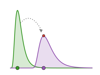
A modifier pipeline

Introduction

The modifiers in this package each wrap one distribution and change one behaviour, and they stack. This tutorial walks a delay distribution through the four verbs in turn: an affine reparameterisation, the forward-series transforms thin and cumulative, the generic series_transform escape hatch, and a hazard modify with both supported links. It closes with get_dist / get_dist_recursive unwrapping a nested stack.

What are we going to do in this exercise

1. Reparameterise a distribution with affine.

2. Attach thin and cumulative to a daily-count series and check they leave the distribution itself untouched.

3. Use the generic series_transform for an arbitrary series map.

4. Modify a hazard through the log and identity links.

5. Peel a nested stack back to its base distribution.

What might I need to know before starting

This tutorial builds on the Getting started overview and uses Distributions.jl and ModifiedDistributions.jl, with CairoMakie and AlgebraOfGraphics for the figures.

Packages used

CairoMakie and AlgebraOfGraphics are used for plotting only.

using ModifiedDistributions, Distributions
using CairoMakie, AlgebraOfGraphics

CairoMakie.activate!(type = "png", px_per_unit = 2)
set_theme!(theme_latexfonts(); fontsize = 14)

Affine reparameterisation

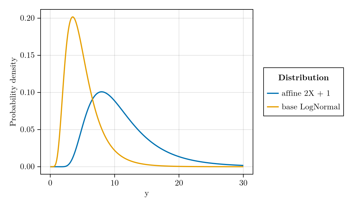
affine gives the exact change-of-variables distribution of Y = scale * X + shift. It reparameterises any univariate distribution uniformly, including families where Distributions.jl has no closed-form affine constructor. The mean printed by the wrapper matches the manual 2 * mean + 1.

base = LogNormal(1.5, 0.5)
scaled = affine(base; scale = 2.0, shift = 1.0)
(affine_mean = mean(scaled), manual = 2.0 * mean(base) + 1.0)

(affine_mean = 11.156838074360163, manual = 11.156838074360163)

Plotting the two densities shows what the transform does: the affine copy is stretched to twice the width, shifted right by one, and half the height, exactly as a change of variables requires.

xs = collect(range(0.0, 30.0; length = 300))
affine_curves = (
    x = vcat(xs, xs),
    density = vcat(pdf.(base, xs), pdf.(scaled, xs)),
    dist = vcat(fill("base LogNormal", length(xs)),
        fill("affine 2X + 1", length(xs)))
)
draw(
    data(affine_curves) *
    mapping(:x => "y", :density => "Probability density",
        color = :dist => "Distribution") *
    visual(Lines, linewidth = 2);
    figure = (size = (600, 350),)
)

The full distribution interface follows the transform, including ccdf computed directly by change of variables rather than via 1 - cdf, so upper-tail probabilities stay precise. The two printed values agree.

x = 6.0
(affine_ccdf = ccdf(scaled, x), manual = ccdf(base, (x - 1.0) / 2.0))

(affine_ccdf = 0.8784793054869964, manual = 0.8784793054869964)

Forward-series transforms on a daily-count series

thin and cumulative do not change the distribution. They carry a deterministic operation intended for a count series that a downstream convolution layer produces, for example an expected incidence curve. The distribution methods stay transparent: logpdf, rand and the rest delegate straight to the base, so the two log-densities printed below are identical.

delay = Gamma(2.0, 1.0)
td = thin(delay, 0.3)          # ascertain 30% of the series
(thinned = logpdf(td, 2.0), base = logpdf(delay, 2.0))

(thinned = -1.3068528194400546, base = -1.3068528194400546)

Sampling is likewise unchanged, because the forward op never touches the distribution: the same seed draws the same value from both.

using Random
(thinned = rand(Random.MersenneTwister(1), td),
    base = rand(Random.MersenneTwister(1), delay))

(thinned = 1.4960845997447596, base = 1.4960845997447596)

The op materialises only when a series is passed through it. The internal hook a convolution layer calls peels the ops off the wrapper and applies them in order; here we drive it directly on a synthetic daily count to show what the op does. Every day in the printed output is 0.3 times the input series.

daily = [0.0, 5.0, 12.0, 20.0, 15.0, 8.0, 3.0]
_, thin_ops = ModifiedDistributions._peel_forward(td)
ModifiedDistributions._apply_forward_ops(daily, thin_ops)

7-element Vector{Float64}:
 0.0
 1.5
 3.5999999999999996
 6.0
 4.5
 2.4
 0.8999999999999999

cumulative accumulates the series into a running total, turning a daily count into a cumulative one — the printed series is the running sum of daily.

cd = cumulative(delay)
_, cum_ops = ModifiedDistributions._peel_forward(cd)
ModifiedDistributions._apply_forward_ops(daily, cum_ops)

7-element Vector{Float64}:
  0.0
  5.0
 17.0
 37.0
 52.0
 60.0
 63.0

The generic series_transform escape hatch

series_transform accepts any callable series -> series, for the cases thin and cumulative do not cover. Here the op shifts every day up by one, as the printed series shows.

shift_op = series_transform(delay, s -> s .+ 1.0)
_, shift_ops = ModifiedDistributions._peel_forward(shift_op)
ModifiedDistributions._apply_forward_ops(daily, shift_ops)

7-element Vector{Float64}:
  1.0
  6.0
 13.0
 21.0
 16.0
  9.0
  4.0

It stays transparent to the distribution in exactly the same way: the two log-densities printed below are identical.

(transformed = logpdf(shift_op, 2.0), base = logpdf(delay, 2.0))

(transformed = -1.3068528194400546, base = -1.3068528194400546)

Hazard modification through a link

modify changes a continuous distribution's hazard through a link. The default log link gives proportional hazards: with effect β and θ = exp(β), the survival function is raised to the power θ. The two printed values agree.

hazard_base = Weibull(1.5, 2.0)
β = 0.5
prop = modify(hazard_base, β; link = log)
(modified = ccdf(prop, 1.0), base_power = ccdf(hazard_base, 1.0)^exp(β))

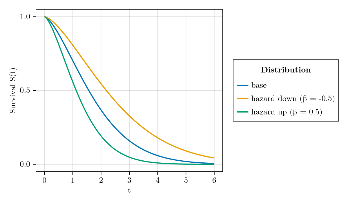
(modified = 0.5582708749558248, base_power = 0.558270874955825)

Plotting the survival functions shows the effect directly: a hazard increase (β = 0.5) pulls the survival curve down, and a hazard decrease (β = -0.5) lifts it above the base.

reduced = modify(hazard_base, -β; link = log)
ts = collect(range(0.0, 6.0; length = 300))
survival_curves = (
    t = vcat(ts, ts, ts),
    survival = vcat(
        ccdf.(hazard_base, ts), ccdf.(prop, ts), ccdf.(reduced, ts)),
    dist = vcat(fill("base", length(ts)),
        fill("hazard up (β = 0.5)", length(ts)),
        fill("hazard down (β = -0.5)", length(ts)))
)
draw(
    data(survival_curves) *
    mapping(:t => "t", :survival => "Survival S(t)",
        color = :dist => "Distribution") *
    visual(Lines, linewidth = 2);
    figure = (size = (600, 350),)
)

The identity link gives additive hazards for a non-negative effect. A constant extra hazard β accrues from the support minimum, so the modified survival is the base survival times exp(-β (t - m)), and the two printed values agree.

add = modify(hazard_base, 0.4; link = identity)
m = minimum(hazard_base)
t = 1.0
(modified = ccdf(add, t), manual = ccdf(hazard_base, t) * exp(-0.4 * (t - m)))

(modified = 0.47069102853491596, manual = 0.47069102853491607)

Both paths are closed form, so the modified distribution samples and integrates like any other.

(sample_mean = mean(rand(prop, 10_000)), cdf_at_2 = cdf(add, 2.0))

(sample_mean = 1.3045402178517709, cdf_at_2 = 0.8347011117784134)

Unwrapping a nested stack

The modifiers nest, and the get_dist protocol peels them back off. get_dist removes one layer; get_dist_recursive keeps going until it reaches a distribution with no more wrappers.

stack = weight(thin(affine(base; scale = 2.0), 0.3), 5.0)
get_dist(stack)          # one layer off: the Transformed wrapper

Transformed(Affine(Distributions.LogNormal{Float64}(μ=1.5, σ=0.5)))

Recursive unwrapping returns the base LogNormal at the bottom of the stack — the very object we started with.

get_dist_recursive(stack)

Distributions.LogNormal{Float64}(μ=1.5, σ=0.5)

Summary

• affine reparameterises any univariate distribution by exact change of variables.

• thin, cumulative and transform stay transparent to every distribution method and act only on a downstream series.

• modify scales a survival curve (log link) or adds a constant hazard (identity link) in closed form.

• get_dist / get_dist_recursive recover the wrapped distribution from any depth of nesting.