Weighted likelihoods

Introduction

weight scales the logpdf contribution of an observation without touching any other distribution method. The wrapped distribution still samples, integrates and reports summary statistics from the base; only the log-density is multiplied by the weight. This is the standard trick for aggregated or count data, where one recorded value stands in for many identical observations.

What are we going to do in this exercise

1. Meet the three ways to supply a weight.

2. See that a weighted distribution still samples from its base, so it stays a complete generative model inside a PPL.

3. See why a zero or missing weight returns -Inf rather than NaN.

4. Compute a weighted log-likelihood surface for aggregated count data with plain Julia, and read the grid maximum off it.

What might I need to know before starting

This tutorial builds on the Getting started overview. It uses Distributions.jl and ModifiedDistributions.jl, so there is no fitting package to install, with CairoMakie and AlgebraOfGraphics for the figure.

Packages used

CairoMakie and AlgebraOfGraphics are used for plotting only.

using ModifiedDistributions, Distributions
using CairoMakie, AlgebraOfGraphics

CairoMakie.activate!(type = "png", px_per_unit = 2)
set_theme!(theme_latexfonts(); fontsize = 14)

The three weight call shapes

A fixed constructor weight

weight(d, w) fixes the weight when the distribution is built. The weighted logpdf is exactly w times the base logpdf, so a value seen w times contributes as if it appeared w times in the sum. The two numbers printed below match.

base = Normal(2.0, 1.0)
wd = weight(base, 25)          # an observation recorded 25 times
(weighted = logpdf(wd, 3.5), manual = 25 * logpdf(base, 3.5))

(weighted = -51.098463330116815, manual = -51.098463330116815)

Everything other than logpdf delegates to the base distribution, so the weight leaves sampling, cdf, quantiles and moments untouched. The mean and cdf of the weighted distribution printed below are those of the base.

(weighted = (mean(wd), cdf(wd, 3.5)), base = (mean(base), cdf(base, 3.5)))

(weighted = (2.0, 0.9331927987311419), base = (2.0, 0.9331927987311419))

A weight supplied at observation time

weight(d) stores a missing constructor weight, so the weight arrives with each observation as a (value = x, weight = w) named tuple. The observation-time weight scales the log-density exactly as the constructor weight did.

wd_obs = weight(base)
(observation_time = logpdf(wd_obs, (value = 3.5, weight = 25)),
    manual = 25 * logpdf(base, 3.5))

(observation_time = -51.098463330116815, manual = -51.098463330116815)

When both a constructor weight and an observation weight are present they multiply. A distribution fixed at weight 2 and an observation weight 3 together contribute six times the base log-density, as the printed pair shows.

(combined = logpdf(weight(base, 2), (value = 3.5, weight = 3)),
    manual = 6 * logpdf(base, 3.5))

(combined = -12.263631199228037, manual = -12.263631199228037)

Vectorised Product forms

Passing a vector of weights builds a Product of weighted components, one per observation. Evaluating its logpdf on a vector of values sums the per-component weighted log-densities, matching the manual weighted sum printed alongside.

counts = [3, 1, 4]
values = [1.9, 2.1, 2.3]
wds = weight(base, counts)
(product = logpdf(wds, values),
    manual = sum(counts .* logpdf.(base, values)))

(product = -7.551508265637382, manual = -7.551508265637382)

The observation-time form vectorises the same way. Building the Product with missing weights and supplying a (values = ..., weights = ...) named tuple applies the weights per element, reproducing the same weighted sum.

wds_obs = weight(fill(base, 3))
(product = logpdf(wds_obs, (values = values, weights = counts)),
    manual = sum(counts .* logpdf.(base, values)))

(product = -7.551508265637382, manual = -7.551508265637382)

Weighted distributions stay samplable

The usual alternatives to weight in a probabilistic programming language are an ad hoc n * logpdf(d, x) term or Turing.jl's @addlogprob!. Both scale the likelihood, but neither leaves behind a distribution the model can sample from. A weighted distribution is still a real Distributions.jl object: sampling delegates to the base while only the likelihood contribution is scaled, so a Turing.jl model (or any PPL built on Distributions.jl) that uses it stays a complete generative model, and prior simulation and posterior-predictive draws keep working. The draws printed below come straight from the base Normal(2, 1).

using Random
rand(Random.Xoshiro(42), wd, 5)

5-element Vector{Float64}:
 2.788355601604292
 1.1201414040456008
 1.126206517790374
 1.2667450355651073
 1.2978048012423196

The sample mean over many draws sits at the base mean, unmoved by the weight of 25, while the log-density at the same point is scaled.

(sample_mean = mean(rand(Random.Xoshiro(42), wd, 10_000)),
    base_mean = mean(base))

(sample_mean = 2.0116769778236603, base_mean = 2.0)

Why zero and missing weights give -Inf

A weight multiplies a log-density, and 0 * logpdf is NaN whenever the base logpdf is -Inf (an out-of-support value). A single NaN poisons a sum and derails a sampler or optimiser, so weight short-circuits a zero or missing weight straight to -Inf, which is the correct log-density of an observation that carries no mass.

logpdf(weight(base, 0), 3.5)

-Inf

The same short-circuit applies to a zero observation weight.

logpdf(weight(base), (value = 3.5, weight = 0))

-Inf

Keeping the branch at -Inf rather than NaN also keeps automatic differentiation well defined, since the poisoned 0 * -Inf product never reaches the gradient.

A weighted log-likelihood surface for aggregated counts

Aggregated count data records each distinct value once alongside the number of times it was seen. Here a delay is measured to the nearest day and tallied.

observed = [2.0, 3.0, 4.0, 5.0, 6.0]
tally = [4, 11, 18, 9, 3]        # counts for each observed value

5-element Vector{Int64}:
  4
 11
 18
  9
  3

The likelihood of a candidate Normal(μ, σ) for the disaggregated data is the weighted sum of per-value log-densities, which the Product form computes in one call.

function grid_loglik(μ, σ)
    d = weight(Normal(μ, σ), tally)
    return logpdf(d, observed)
end

grid_loglik (generic function with 1 method)

Sweeping μ over a grid at a fixed σ traces the profile log-likelihood. No fitting package is needed: the grid maximum is the maximum-likelihood μ on the grid.

μ_grid = range(3.0, 5.0; length = 21)
σ_fixed = 1.2
surface = [grid_loglik(μ, σ_fixed) for μ in μ_grid]

21-element Vector{Float64}:
 -79.07059293882713
 -76.3796207166049
 -74.00114849438268
 -71.93517627216046
 -70.18170404993825
 -68.74073182771602
 -67.61225960549379
 -66.79628738327156
 -66.29281516104935
 -66.10184293882713
   ⋮
 -67.40392627216046
 -68.46295404993823
 -69.83448182771602
 -71.51850960549379
 -73.51503738327156
 -75.82406516104936
 -78.44559293882713
 -81.37962071660492
 -84.62614849438269

The best grid point sits where the surface peaks.

best = argmax(surface)
(μ_hat = μ_grid[best], loglik = surface[best])

(μ_hat = 3.9, loglik = -66.10184293882713)

Plotting the surface over the grid shows the peak in context: the curve rises to a single maximum (marked) and falls away on either side.

surface_curve = (μ = collect(μ_grid), loglik = surface)
peak_point = (μ = [μ_grid[best]], loglik = [surface[best]])
draw(
    data(surface_curve) *
    mapping(:μ => "μ", :loglik => "Weighted log-likelihood") *
    visual(Lines, linewidth = 2) +
    data(peak_point) *
    mapping(:μ => "μ", :loglik => "Weighted log-likelihood") *
    visual(Scatter, markersize = 12, color = :black);
    figure = (size = (600, 350),)
)

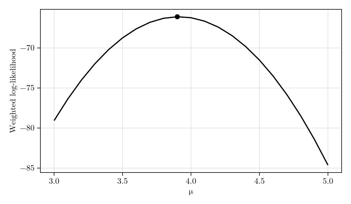
The grid estimate matches the count-weighted sample mean, the closed-form maximiser for a Normal mean, up to the grid spacing. The two printed values agree to within half a grid step.

weighted_mean = sum(tally .* observed) / sum(tally)
(grid_estimate = μ_grid[best], weighted_mean = weighted_mean)

(grid_estimate = 3.9, weighted_mean = 3.911111111111111)

Summary

• weight(d, w), weight(d) with (value =, weight =), and the vectorised Product forms cover fixed, observation-time and per-element weights.

• A weighted distribution still samples from its base, so a Turing.jl model using it stays a complete generative model with working prior and posterior-predictive simulation.

• A zero or missing weight returns -Inf, keeping the log-density and its gradient well defined.

• A weighted Product turns aggregated counts into a single logpdf call, enough to trace a log-likelihood surface and read off a grid estimate with plain Julia.

• To weight the observed total of a composed chain of delays, see the Modifiers across composed chains tutorial.