Getting started

Welcome to the ModifiedDistributions documentation. This page is the quickstart: what the package is for, how to install it, and a tour of each modifier.

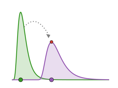
ModifiedDistributions provides modifiers for Distributions.jl univariate distributions. A modifier is a wrapper around exactly one distribution that changes one behaviour, returning something that still works anywhere a distribution is expected. Modifiers nest freely, and the get_dist protocol unwraps them again.

Installation

See the Installation page for setup, then load the package alongside Distributions.jl:

using ModifiedDistributions, Distributions

A composed pipeline

Modifiers nest, so a real pipeline stacks several changes on one delay: an intervention that halves the hazard of admission, a half-day reporting lag, and a 60% ascertainment fraction tagged for a downstream count series.

admission = Gamma(2.0, 1.0)   # baseline infection-to-admission delay

pipeline = thin(affine(modify(admission, -log(2.0)); shift = 0.5), 0.6)

Transformed(Affine(Modified(Distributions.Gamma{Float64}(α=2.0, θ=1.0), -0.6931471805599453; link=LogLink)))

pipeline prints as the nested wrapper it is.

pipeline

Transformed(Affine(Modified(Distributions.Gamma{Float64}(α=2.0, θ=1.0), -0.6931471805599453; link=LogLink)))

Each stage compounds the three-day survival: halving the hazard raises it to its square root, and the reporting lag raises it further (day 3 is now effectively day 2.5 post-admission); thin does not touch the scalar distribution at all, only tagging it for later use against a count series.

(baseline_survival = ccdf(admission, 3.0),
    after_intervention = ccdf(modify(admission, -log(2.0)), 3.0),
    after_reporting_lag = ccdf(pipeline, 3.0))

(baseline_survival = 0.19914827347145578, after_intervention = 0.44626032029685964, after_reporting_lag = 0.536001394759049)

Unwrapping recovers the baseline delay underneath every layer.

get_dist_recursive(pipeline) == admission

true

The rest of this page tours each modifier on its own, and the Extensions section below shows what thin does once it meets a real count series.

Affine transforms

affine gives the exact change-of-variables distribution of Y = scale * X + shift:

d = affine(LogNormal(1.5, 0.5); scale = 2.0, shift = 1.0)
(mean = mean(d), logpdf = logpdf(d, 5.0), median = quantile(d, 0.5))

(mean = 11.156838074360163, logpdf = -2.914108658241349, median = 9.963378140676129)

The full distribution interface works, including sampling and ccdf/logccdf computed directly rather than via 1 - cdf, so upper-tail probabilities stay precise.

Likelihood weights

weight scales the logpdf contribution of an observation, which is the standard trick for aggregated or count data. The two numbers printed below match, showing the weighted log-density is exactly 25 times the base:

base = Normal(2.0, 1.0)
wd = weight(base, 25)  # an observation seen 25 times
(weighted = logpdf(wd, 3.5), manual = 25 * logpdf(base, 3.5))

(weighted = -51.098463330116815, manual = -51.098463330116815)

Weights can also arrive at observation time, or vectorised as a Product distribution:

wd_obs = weight(base)  # weight supplied with the observation
logpdf(wd_obs, (value = 3.5, weight = 25))

-51.098463330116815

wds = weight(base, [3, 1, 4])
logpdf(wds, [1.9, 2.1, 2.3])

-7.551508265637382

Everything other than logpdf (sampling, cdf, quantiles, summary statistics) delegates to the underlying distribution, so a weighted distribution stays a complete generative object in a probabilistic programming model.

Forward-series transforms

thin and cumulative attach a deterministic operation intended for a downstream count series (for example, one produced by a convolution layer): thinning by an ascertainment probability, or accumulating to cumulative incidence. They are transparent to every distribution method, so the two log-densities printed below are identical:

td = thin(Gamma(2.0, 1.0), 0.3)
(thinned = logpdf(td, 2.0), base = logpdf(Gamma(2.0, 1.0), 2.0))

(thinned = -1.3068528194400546, base = -1.3068528194400546)

The generic series_transform accepts any callable series -> series as an escape hatch. thin and cumulative cover the common cases; series_transform takes any callable series -> series.

Hazard modification

modify changes a continuous distribution's hazard function through a link. Under proportional hazards the survival function is raised to the power exp(effect), and the two values printed below agree:

base = Weibull(1.5, 2.0)
md = modify(base, 0.5)  # proportional hazards: h*(t) = exp(0.5) * h(t)
(modified = ccdf(md, 1.0), base_power = ccdf(base, 1.0)^exp(0.5))

(modified = 0.5582708749558248, base_power = 0.558270874955825)

The default log link gives proportional hazards; link = identity gives additive hazards for non-negative effects.

Unwrapping

Modifiers nest, and get_dist / get_dist_recursive peel them back off:

nested = weight(affine(Normal(0, 1); scale = 2.0), 3.0)
(get_dist(nested), get_dist_recursive(nested))

(Affine(Distributions.Normal{Float64}(μ=0.0, σ=1.0)), Distributions.Normal{Float64}(μ=0.0, σ=1.0))

Downstream packages can extend get_dist for their own wrappers to join the same protocol.

Extensions

Loading ComposedDistributions.jl alongside this package activates an extension that lets the modifier verbs apply to a composed Sequential chain, modifying the one scalar quantity the chain observes (see the Modifiers across composed chains tutorial for why there is exactly one observed scalar):

using ModifiedDistributions, ComposedDistributions, Distributions

chain = sequential(:onset_admit => Gamma(2.0, 1.0),
    :admit_death => LogNormal(0.5, 0.4))
wd = weight(chain, 3.0)  # weights the chain's observed total
logpdf(wd, 5.0)          # 3 times the log-density of the observed total

The extension in this package handles applying modifiers to a chain; the reverse direction — rewrapping modifier leaves inside a chain — lives in ComposedDistributions.jl. See the Modifiers across composed chains tutorial for a worked example.

Loading ConvolvedDistributions.jl activates a second extension. Its series verb convolve_series(delay, series) turns an expected-events series into expected downstream counts, and the extension makes the forward-series transforms act on those counts: thin rescales them by an ascertainment fraction, cumulative accumulates them, and series_transform applies any callable. It also lets the modifier wrappers serve as components of a distribution-level convolution, including under automatic differentiation:

using ModifiedDistributions, ConvolvedDistributions, Distributions

total = convolved(Gamma(2.0, 1.0), LogNormal(0.5, 0.4))
infections = [0.0, 10.0, 40.0, 90.0, 60.0, 20.0]
convolve_series(thin(total, 0.3), infections)  # 30% ascertained counts

See the Convolving modified distributions tutorial for a worked example.

Learning more

• Want the full interface? See the Public API.

• Common questions are answered in the FAQ.

• Writing your own wrapper? See Writing a new modifier.

• Want the packages ModifiedDistributions works alongside? See Related packages on the home page.

Getting help

For usage questions, ask on the Julia Discourse (the SciML or usage categories) or the epinowcast community forum, our home for epidemiological modelling questions. Please use GitHub issues for bug reports and feature requests only.